josh's site

Writing a Chess Engine: Move Selection

12/17 - 2022

This is the second of two-part article about my experience writing a chess engine from scratch. I highly recommend reading the first post about move generation. This post will focus on move selection - given a position and a list of all possible moves we can make, how do we decide which move is best?

The Minimax algorithm

Let’s begin with the fundamental algorithm that the rest of our engine will be built up - the minimax algorithm. The minimax theorem was proven by John von Neumann (the same guy who worked on the atomic bomb and did work on linear programming) in 1928, and is a foundational part of game theory.

A core piece of this algorithm is the idea of an evaluation - this is some numerical value which represents the strength of a chess position. By convention, we say that negative values are better for black, positive values are better for white, and a value of zero is a draw.

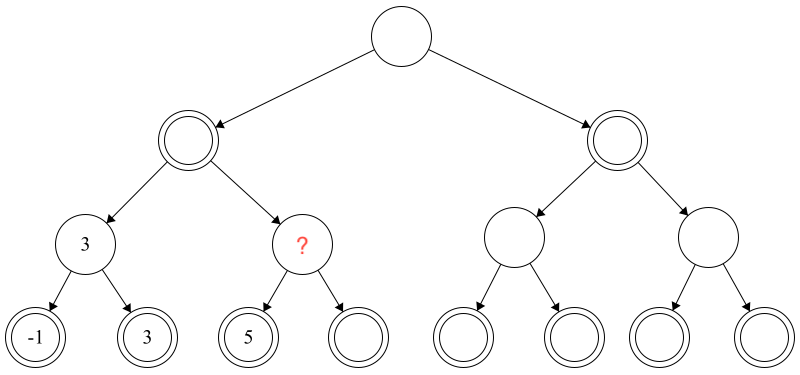
Pictured below is a tree which represents the possible paths that a game can take, up to an arbitrary depth of three. This doesn’t represent a real chess game, but rather a simplified version for the sake of learning.

At the leaf nodes, we’ve done some sort of analysis (we’ll talk about this in more detail later), and assigned each position a value based on it’s evaluation. The bottom left-most node has a value of -1, meaning it’s winning for black. The right-most node has a value of 9, meaning that it’s very winning for white. Note that the circles in this picture have either single or double borders. Single borders means white moves at that level, double borders means that its blacks move.

This tree represents something that the player with the white pieces would calculate for the minimax algorithm in a certain position, since they are the player at the root node. First, we enumerate all moves up to a certain depth and evaluate the strength of the position at the leaf nodes only.

The next step is determining, for each parent node of the leaf nodes, which value should go there. Since the parent of these nodes is a move for white, this means that we should populate each node with the maximum value of our children. This is because it’s white’s turn to move, and so we should pick the move that’s best for us. So, at the next stage, our tree would look something like this:

Now, we repeat the previous step for the nodes one level higher with a slight modification - we are now minimizing the value of our children. That is because, at this step, we are considering moves as the black pieces. Since black is trying to minimize their score, we should assume that black will play optimally and will always pick the lowest evaluation of it’s children. So, after this step, our tree will look like this:

We repeat once again for the root node. Since this node is a move for white, we pick the maximum value of our children and arrive at the following tree:

What this tells us is that, looking three moves ahead, we will be able to guarantee a position which has an evaluation of 3. It’s possible that we can do even better since black might not play optimally. But, in the worst case, white is guaranteed a value of three.

At the point we can understand how the algorithm gets it’s name - at each step we are trying to populate the value of nodes such that we maximize the minimum gain.

Let’s go ahead and write some pseudo-code for the minimax algorihtm:

func minimax(Board b, uint depth):
    if depth == 0 or there are no legal moves:
        return evaluation(b)

    let val
    if b.is_white_to_move():
        val = -inf
        for each move in b:
            val = max(val, minimax(board.apply(move), depth - 1)
    if b.is_black_to_move():
        val = inf
        for each move in b:
            val = min(val, minimax(board.apply(move), depth - 1);

    return val

Alpha-Beta Pruning

While the minimax algorithm is a nice theoretical foundation for our engine, it will not give us a strong engine on it’s own. Recall that the first step in our algorithm was enumerating all legal moves up to some arbitrary depth. Even though modern computers are very fast, chess is still a very complicated game with a very high branching factor. On any given turn, there are on average about 30 moves that a player can make. Because of this, getting a minimax engine to efficiently search to a depth of more than 6 or 7 on every move is simply infeasible. Note that the world’s top engines (like Stockfish), are able to routinely search to depths in the mid 20s - so how do they do it?

A natural first question to ask is “well, do we have to search all of these nodes?” (in general, I find that “is this something we even need to do” is a great question to ask as an engineer). The answer, probably unsurprisingly, is no. The reason for this, however, is a bit more difficult to start. To see where our inefficiencies lie, let’s take a snapshot midway through the minimax algorithm. We’ll use the same game tree from before and we’ll start evaluating the same way - evaluate some leaf nodes and then determine the value of the parent.

Now, at this stage, our algorithm will be considering the value of the parent node of 5. Ask yourself this question - do we need to evaluate the value of the leaf node adjacent to 5? The answer is no - but why? To see this, we have to look beyond just our current node/children and consider the whole search so far. Because the node we’re looking at is a move for white, we know that we’re going to be maximizing our search. And, because we have already seen a value of 5, we know that the value of the current node is some value greater than 5. Furthermore, we’ve already searched the node to our left which has a value of 3. This means that our parent node will be deciding between two values: 3 and some value that is greater than or equal to 5. But our parent node is the minimizing player, which means that they’re going to pick the smallest of the two values presented. And, since our value is at least five, there are no circumstances under which they would pick our branch. Because of this, we can stop searching on this branch.

This optimization is something called alpha-beta pruning. Unlike the minimax algorithm, we do our search depth-first (meaning we evaluate one position all the way to the leaf nodes). As we go, we keep track of two values - alpha and beta. Alpha represents the best value that white is guaranteed, while beta represents the best value that black is guaranteed.

In this previous example, alpha would have a value of 3 (the best score white is guaranteed so far), while beta would have a value of 5 (the best score black is guaranteed). Since alpha has exceeded beta, we can conclude our search.

Alpha-beta pruning allows us to prune large sections of the tree and achieve much greater search depths than we would with a minimax search. A basic pseudocode outline of alpha-beta pruning is as follows:

func alpha_beta(Board b, int alpha, int beta, uint depth):
  if depth == 0 or there are no legal moves:
    return evaluation(b)

  let val
  if b.white_to_move():
    val = -inf
    for each move in b:
      val = max(val, alpha_beta(b.apply(move), alpha, beta, depth -1))
      if eval >= beta:
        break
      alpha = max(alpha, val)
  if b.black_to_move():
    val = inf
    for each move in b:
      val = min(val, alpha_beta(b.apply(move), alpha, beta, depth - 1))
      if eval <= alpha
        break
      beta = min(beta, val)

  return val

Alpha-Beta vs. Minimax metrics

It’s one thing to claim that alpha-beta pruning offers a performance improvement over minimax - but how much does it really? There are numerous factors at work with regards to how much better alpha-beta performs than minimax (more on that later), but let’s compare some baseline numbers to understand how these algorithms compare.

A good metric to use when comparing these two algorithms is how many evaluations we need to perform. Although we haven’t talked much about evaluation functions yet, we want to ultimately minimize the number of times we analyze our position and generate a value that represents its strength for each player.

From the starting position, here are the number of positions that each algorithm must evaluate at each depth:

Depth  Minimax  Alpha-Beta
  
  1         20          20
  2        400          39
  3       8902         524
  4     197281        1229
  5    4865617       32138

Iterative-Deepening & Transposition Tables

Despite the performance improvements that alpha-beta pruning offers over minimax, it still is only able to achieve modest search depths at best. Even on my most modern hardware, searching to depth 7 from the starting takes about 3.5 seconds, and depth 8 takes about 37 seconds. There are still a few problems with our engine, however.

The first issue is that our engine is going to do a poor job of time management. If we simply always instruct our engine to go to depth 7, we might achieve it in less time than expected and lose out of searching deeper. If we instruct our engine to go deeper - say depth 8 - then we risk running out of time and losing to our opponent.

The second issue, which ends up leading to a solution for the first issue, is that we’re doing a lot of extra work on each search. If you’ve ever studied chess openings, you might be familiar with the term “transpose.” A transposition is the same position in chess which can be reached in numerous ways. Consider the following position, for example:

There are numerous ways to achieve this position. Two of them, for example

1 nc3 Nc6
2 nf3 Nf6

or

1 nf3 Nc6
2 nc3 Nf6

Regardless of how we reached this position, the evaluation will be the same (keep in the mind that the “position” is a term that includes not just the pieces on the board, but also the castling rights of each player and which file an en passant capture is possible, if any).

As such, it would be very helpful if we had some sort of data structure that remembered previous positions. Chess engines solve this problem using something called a transposition table - a specialized hash table which maps positions to their evaluations so that they can be reused.

One of the major benefits of a transposition table will be to solve our time management strategy using something called iterative deepening. The idea behind this is to first search to depth 1, then depth 2, then depth 3… until you run out of time. Should you be interrupted mid search, you can always fall back to the previous depth search. And, since positions are cached, searching to depth 7 after depth 6 is almost trivial.

Zobrist Hashing

Although it may be tempting to use a pre-made HashMap (perhaps from Rust’s standard library), there are a few reasons we might want to implement our own transposition table.

• Bounded capacity - if we store a unique entry for every position we see, we’ll quickly create an unreasonably large table.
• More control over keys - storing the entire position struct as a key would be undesirable, as it would take up too much space. We’ll need to implement our own hashing algorithm.
• More control over collisions - Our table is going to have a lot of collisions given the volume of entries we’re inserting and the constrained size of our table. We need to have control over when a fetch is valid and when we can evict previous entries in favor of new ones.

Since we’re implementing our own table, we should also implement our own hashing algorithm. Our algorithm should have two main properties

1. Keys should lightweight (preferably 64-bits)
2. Altering a position’s key based on a single move should be very fast.

The most common approach to generating such keys is using a technique called Zobrist hashing. Zobrist hashing is a technique that produces particularly good keys for a chess engine, since the hashes are very evenly distributed while also being very quick to generate and manipulate.

The general idea of the algorithm is quite simple. We start by generating a random 64-bit integer for each unique triplet of

1. The square (A1, A2,..)
2. The type of piece (Rook, Bishop,…)
3. The color

as well as a random number for the file that can be captured en-passant, four random numbers for the castling rights, and one for the active player. In other words, each piece of information that could define the game state is given its own random number.

To generate a hash for a given position, we simply take the XOR of all the 64-bit numbers that represent that position. Not only is this operation very fast, but it’s also very quick to undo. Once you make a move on a position, you can simply XOR out the random number that was affected (this is possibly because the XOR operation is it’s own inverse).

Transposition Table

Given that we can produce a 64-bit hash based on a given position, let’s start implementing a basic transposition table. Let’s start with a basic skeleton and address some more complicated parts from there.

pub struct Entry {
    pub best_move: EvaledMove,
    pub hash: u64,
    pub depth: u8,
}

pub struct TranspositionTable {
    table: Vec<Option<Entry>>,
}

impl TranspositionTable {
    pub fn new_mb(size: usize) -> TranspositionTable {
        let size = size * 1024 * 1024 / mem::size_of::<Entry>();
        Self::new(size)
    }

    pub fn save(&mut self, hash: u64, entry: Entry) -> bool {
        let index = hash as usize % self.table.len();
        self.table[index] = Some(entry);
        true
    }

    pub fn get(&self, hash: u64) -> Option<Entry> {
        let index = hash as usize % self.table.len();
        let entry = self.table[index];
        if (entry.is_some() && entry.unwrap().hash == hash) {
            return Some(entry);
        }
        None
    }
}

So far this implementation is fairly straightforward, clients of our table can save entries in the table and retrieve them. There are a few considerations we must make going forward, however.

The first issue is that our table will actually return incorrect results to us. The reasoning for this, however, is quite difficult to spot. Suppose that we are searching at the root node of our tree and lookup the current position in the table. Assuming we get a hit, are we able to return that value and claim that is the evaluation of our position? The answer is no, since whatever value we fetched was found somewhere lower down the tree, meaning it was constructed with less information than we currently have available to us. Thus, anytime we try to fetch a value from our table, we are only able to do so if the value that we’re fetching was found at the same level, or higher up the tree, than our current position. In code, this would look something like this:

--pub fn get(&self, hash: u64) -> Option<Entry> {
++pub fn get(&self, hash: u64, depth: u8) -> Option<Entry> {
--if (entry.is_some() && entry.unwrap().hash == hash) {
++if (entry.is_some() && entry.unwrap().hash == hash && entry.depth >= depth) {
    return Some(entry);
}

The second issue is a replacement strategy. Even with a large table (something on the order of hundreds of megabytes), we are still going to run into lots of collisions. If we have two entries that map to the same index, how do we decide which one goes there? A very simple solution is an “always-replace” strategy. In essence, given any position, we simply always overwrite the position that is currently there. However, we can use our knowledge from the first problem we had to come up with a better replacement strategy. Entries that are searched near the leaves of the tree are not very valuable, since we just determined that entires closer to the root are based off of more information. And since they’re fetched closer to the root, we’re more likely to see those positions closer to the root in the future, allowing us to avoid searching large swaths of the tree. This leads us to another strategy - only replace nodes if the depth of the incoming entry is greater than, or equal to, the depth of the existing entry (recall that depth is a somewhat counter-intuitive number in that root nodes have a depth of n and leaf nodes have a depth of 0).

pub fn save(&mut self, hash: u64, entry: Entry) -> bool {
  let index = hash as usize % self.table.len();
  let prev_entry = self.table[index];
  if prev_entry.is_none() {
    self.table[index] = Some(entry);
    return true;
  } else if prev_entry.is_some() && 
      prev_entry.unwrap().depth <= depth {
    self.table[index] = Some(entry);
    return true;
  }
  false
}

Now that we have a transposition table implemented for alpha-beta pruning, lets do a comparison against the original implementation and see how much better it performs in terms of nodes searched.

Depth  Alpha-Beta   Alpha-Beta w/ TT
  
  3           524                 63        
  4          1229                 82
  5         32138               1036
  6        723278               3707
  7       1074965               6104
  8      32521084              24623
  9      93555968              33294
 10    1886549650             333591

Iterative deepening

Now that we have a transposition table implemented, we can go ahead and implement iterative deepening. This is a very simple concept, it is our engine’s primary time-management strategy while providing near identical performance to just searching to the provided depth directly. The pseudocode is quite simple:

func best_move_itr_deepening(pos, depth):
    best_move := null move
    for i in 0 to depth:
        best_move = alpha_beta(pos, -INF, INF, depth)

    return best_move

In other words, we first search to depth zero, then depth 1, all the way until depth n rather than going to depth n initially.

The Horizon Problem

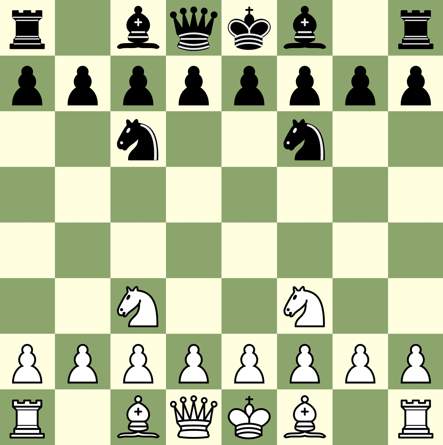
If you’ve been following along carefully, you might have already found one flaw in our engine. To discover what this is, let’s consider a relatively simple position (white to move)

Now lets say, just for the sake of learning, that we evaluate alpha-beta pruning up until depth 1 (looking just one move ahead. Surely Qxd6+ looks like a nice move - after all we’re winning a rook! Had we looked one move deeper we would have realized we just traded a queen for a rook - which is a bad trade in this instance!

This highlights something called the horizon problem - if we only ever look to a certain depth, we’re inevitably going to run into situations where our evaluation is inaccurate based on some move just a few depths deeper. To remedy this problem, most chess engines do something called a quiescence search (try spelling that 10-times fast). Instead of doing a static evaluation when our alpha-beta search reaches depth zero we instead perform a modified alpha-beta search. The key difference here is that we filter on moves that are captures-only. The goal is to get to a “quiet” position - one where there are no more captures, so that we can be sure we aren’t blundering a piece to some tactic.

In terms of code, we would modify our alpha-beta algorithm like so:

--if depth == 0 or there are no legal moves:
--    return evaluation(b)
++if there are no legal moves:
++    return evaluation(b)
++if depth == 0
++    return q_search(b)

Evaluation Functions

Let’s now talk concretely about evaluation functions - functions which take in a static position and return a number representing how good that position is for each player (recall that, by convention, positive numbers are winning for white while negative numbers are winning for black).

In the world of alpha-beta-type chess engines, there are two prevailing static evaluation functions. Handcrafted functions, which we’ll be using, use a number of fine-tuned human-created heuristics to evaluate a position. Neural networks, which Stockfish started using primarily in 2020, use machine learning to evaluate positions based on large amounts of training data. While learning about neural networks here does sound enticing, let’s limit the scope of the project for now and use hand-crafted evaluation functions.

Handcrafted evaluation functions rely heavily on fundamental chess principles. If you’ve ever read Jeremy Silman’s and Yasser Seirawan’s Play Winning Chess, then many of the heuristics we’ll mention here will be familiar to you.

First and foremost, we will use material difference to evaluate a position. This part of the function simply takes the difference between the number of pieces for each player, and multiplies each by the value of that piece. As is generally accepted, pawns are worth one point, knights and bishops three points, rooks five points, and queens nine points. Some engines give artificially high values to the king to get around generating all legal moves (if the king is captured, it is considered very bad and so legality is determined in alpha-beta pruning).

One edge case we must consider is whether or not the position results in a checkmate. This can be inferred by the number of legal moves in a position, and results in a very positive or very negative value.

Another commonly used heuristic is a piece-square table. This maps a piece and a square to a given value, providing a fast approximation for how good a piece is going to be on that square. The piece-square table for a knight would look something like this:

-50 -40 -30 -30 -30 -30 -40 -50 
-40 -20   0   0   0   0 -20 -40 
-30   0  10  15  15  10   0 -30 
-30   5  15  20  20  15   5 -30 
-30   0  15  20  20  15   0 -30 
-30   5  10  15  15  10   5 -30 
-40 -20   0   5   5   0 -20 -40 
-50 -40 -30 -30 -30 -30 -40 -50 

As you can see, this incentivizes our engine to place nights on centralized squares and towards our opponent’s side of the board.

From here, there is really no limit to how in-depth we can make our evaluation function. Some other common heuristics we could add are:

• Mobility (the number of legal moves the current player has)
• Center control (how many pieces occupy or attack the center of the board)
• Space (how many safe squares minor pieces might move to)
• etc

As I’ll discuss later, evaluation functions are really a black-hole of time and complexity when it comes to working on an engine. You can make a surprisingly good engine using just material difference and piece-square tables, so this is a good place to start while you finish up other parts of the engine.

Optimizations

At this point, we have a functional searcher which incorporates the fundamental components of most modern engines. As we’ll soon see, however, chess engines are really a black-hole of complexity, and there are always other features we can add to improve playing strength.

Speaking generally, the primary strategy for improving playing strength is by reducing the number of nodes our engine must consider - allowing us to spend more time looking deeper into a position.

Move Ordering

The first strategy that we’re going to look at is something called move ordering. If you consider the alpha-beta algorithm, you might notice that the number of positions it searcher differs depending on what order the nodes are looked into. Generally speaking, it is almost always worth it to spend time sorting moves rather than exploring the tree as any early cutoffs we can achieve will have massive impacts on our engine’s ability to search to greated depths.

One of the most common move-ordering heuristics is called MVV-LVA - Most Valuable Victim, Least Valuable Attacked. The idea is quite simple - moves in which low value pieces (i.e. pawns) take high value pieces (i.e. queens) are likely to be good moves and as such should be searched first. In this heuristic, we can use a table to enumerate all possible capture and sort them above non-captures.

In addition to general move ordering, there are two useful techniques for sorting the first move in a given position.

The first technique is trivial to implement and involves using our TT. If you recall from the previous TT section, even though we have an entry for a position in our TT does not mean that we can immediately return the saved best move in the table since it might have been found at a shallower depth. However, it is still likely to be the best move in the position, and so it is reasonable to search it first if such a move exists.

The next technique is called Internal Iterative Deepening. Much like the TT method, this technique is quite trivial to implement. In short, if the TT lookup returned no best move for the current position, and we are on a PV-Node (i.e. a left-most node in the tree), then we can estimate a best move by doing a regular alpha-beta search at a reduced depth (often depth / 2). Since PV nodes are rare, and we are likely to get good TT results with an internal search, it is worth the extra time to do this lookup.

Late Move Reduction

Coming soon…