Computational Photography: Image Stitching

12/25 - 2022

Introduction

Over the last year, I’ve become very interested in film photography. It’s a wonderful way to engage with a hobby that doesn’t primarily involve computers (yes, I understand the irony of writing about film photography on my computer). This last summer I moved from Seattle to San Francisco, and each Sunday I would take my camera and a fresh roll of film and take photos of a new part of the city. The limited number of photos you can take really forces you to slow down and appreciate the world around you.

This last week I took my camera to the Outer Richmond to take some photos at golden hour and watch the sunset. Just as the sun was setting, I took this photo.

Figure 1

While a photo of my white converse taken on a film camera in San Francisco is quite indie, what would really maximize the indie-ness of this photo was if you could see the borders of the film. In other words, this photo.

Figure 2

However, getting this image is not trivial. After I develop my negatives, I use a Plustek scanner to get digital copies. This scanner, however, is specifically designed to only scan exactly the size of a 35mm negative, meaning that the border is not included in the scan.

To get around this, I tried slightly offsetting the negative in the scanner such that it would return a scan of the corner of the negative, including the sprockets around the exposure. Doing this for each corner, I got the following four images.

Figure 3

This article will explore how we can take the four images in Figure 3 and programmatically combine them into the image in Figure 2.

Algorithmic Intuitions

The problem that we’re attempting to solve here is a well known one in computer vision, and is referred to formally as image stitching. Most people have likely used image stitching at some point - taking a panorama photo on your smartphone is just one example. The idea is quite simple - take a series of overlapping photos and stitch them together such that the images “line up” the best they can.

Let’s start to imagine a solution to this problem as if we weren’t writing a program. If someone gave you two partially overlapping photos and asks you to line them up, you would probably begin by identifying certain features which are easy to align. In Figure 3, for example, you might try lining up the red line on my shoes as they’re fairly distinct and easy to tell when they line up.

Feature Identification Using Harris Corners

Let’s start by identifying features more formally in our source images using Harris corner detectors. To fully understand how these detectors work, however, we’ll need to backtrack to some of the fundamental building blocks of computer vision.

Computer Vision Fundamentals: Matrices & Kernels

At the most basic level, we can think of a greyscale image as some matrix \(A\) where each value in \(A\) represents the intensity of light at that location in the image. Most greyscale images use 8-bit values, meaning that each pixel has a value somewhere between 0 and 255. For the rest of this article we’ll assume that all images are greyscale, which can usually be done without a loss of generality.

A kernel, sometimes called a mask, is a small matrix which is used to modify an image. Some example uses of kernels are edge/ridge detection, sharpening, and blurring. A kernel \(\omega\) is applied to a source \(A\) using an operation called a convolution rather than a traditional matrix multiplication (although it is usually still denoted with the * operator).

Convolutions: Theory

Let’s use a concrete example to explain how a convolution works before defining it more formally. Let’s define our convolution \(\omega\) and our source matrix \(A\)

We start by centering the kernel at the top left of the source and sum all products of the overlapping elements between the source and kernel. We then shift the kernel over all elements of the source until we’ve generated a complete target image. Let’s see what this operation looks like for the highlighted source value. We define \(g(x, y)\) as the output image and \(a(x, y)\) as the input matrix for some arbitrary coordinates \(x\) and \(y\).

Performing the convolution over the entire source matrix would give us the following output

Convolutions: Examples

Depending on the kernel used, we can achieve different results with our convolution. Below, I provide some examples of different kernels and their impact on the source image.

Operation	Kernel	Output
Identity	\(\begin{pmatrix} 0 & 0 & 0 \\ 0 & 1 & 0 \\ 0 & 0 & 0\end{pmatrix}\)
Blur	\(\frac{1}{9}\begin{pmatrix} 1 & 1 & 1 \\ 1 & 1 & 1 \\ 1 & 1 & 1\end{pmatrix}\)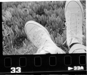
Sharpen	\(\begin{pmatrix} 0 & -1 & 0 \\ -1 & 5 & -1 \\ 0 & -1 & 0\end{pmatrix}\)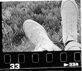

Harris Corner Detectors

As we stated earlier, the first step in combining images is going to be identifying features that we will eventually be able to “line up”. Corners are especially good features to look for since they are rotationally invariant. If you rotate an image by some amount, the vertical and horizontal edges will be drastically changed and become difficult to align (especially for a dumb computer). Corners, however, don’t have this property and as such are good first candidates for extracting features from images.

Computing Gradients

To compute corners, let’s start by producing two output images which emphasize the vertical and horizontal lines on our source image. This operation uses the Sobel operator, which involves the following two kernels.

If we apply these kernels to the bottom-left image of Figure 3, we achieve the following results.

Operation	Kernel	Output
Horizontal Derivative	\(\begin{pmatrix} 1 & 0 & -1 \\ 2 & 0 & -2 \\ 1 & 0 & -1\end{pmatrix}\)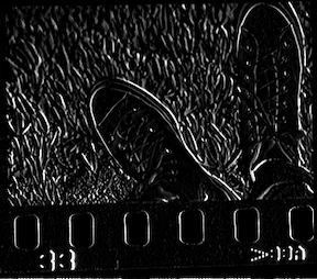
Vertical Derivative	\(\begin{pmatrix} 1 & 2 & 1 \\ 0 & 0 & 0 \\ -1 & -2 & -1\end{pmatrix}\)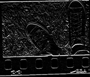

We then formally define \(I_X\) and \(I_y\) as the matrices resulting from performing these two convolutions on the source image.

Identifying Corners Using Gradients

Now that we have two matrices which identify gradients in the \(x\) and \(y\) directions, we can use this information to identify corners. Doing so, however, requires a key observation - corners are elements of our image which contain gradients in both the \(x\) and \(y\) directions.

One way to visualize this is to imagine a plot in \(I_x\) and \(I_y\) space (recall that these two matrices represent the gradient in the \(x\) and \(y\) directions, respectively). Picture the following three scenarios and what the respective plots on the \(I_x\) and \(I_y\) axis would look like

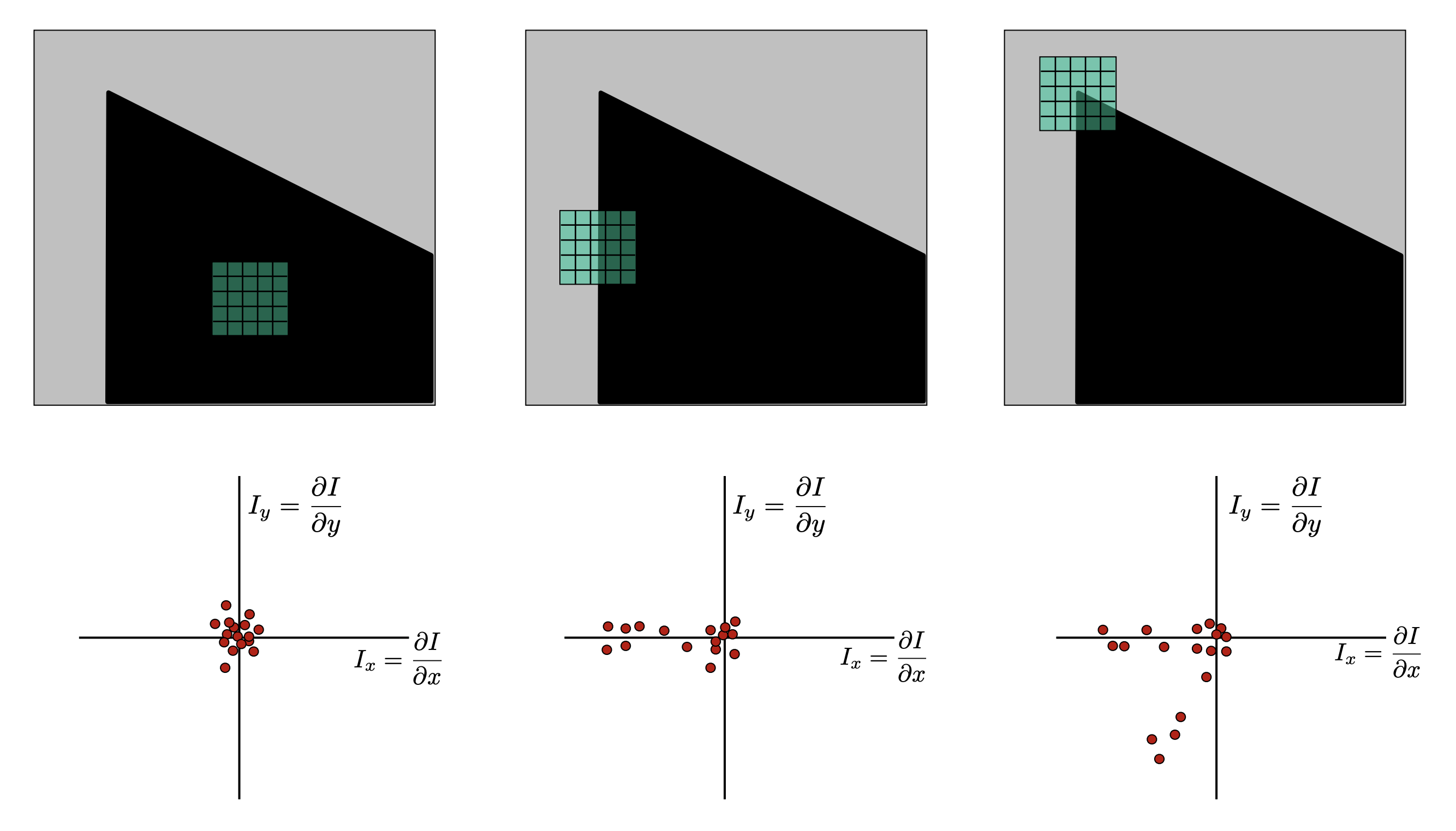Figure 4, courtesy of Kris Kitani at CMU

Speaking generally, there are three separate cases

• Generally smooth regions will have all elements around the origin
• Edges will have elements which extend around a single vector
• Corners will have elements which extend around two vectors

If you have some background in applied mathematics you might quick recognize this as a problem very similar to PCA - principle component analysis. Here, we can imagine that PCA is used to determine in how many dimensions our data is distributed. If it’s distributed in two we have a corner, otherwise we have an edge or a generally smooth region of our image.

We now have a general strategy moving forward - let’s start by summarizing the gradient information at each pixel of our image and then compute how corner-like that gradient is. This involves creating a new matrix, we’ll call it \(M\) such that each entry of \(M\) is defined as follows

I glossed over some of the finer details here, but \(S_{x^2}\), \(S_{xy}\), and \(S_{y^2}\) are matrices who elements are simply weighted average of the gradient around each pixel. Note that \(M\) has been deliberately chosen since it represents the covariance of our two variables - the gradient in the \(x\) direction and the gradient in the \(y\) direction.

With our covariance matrix in place, it’s time to determine to what extent our image has gradients in the two directions. Much like PCA, this information is encoded as the eigenvalues and eigenvectors of the covariance matrix \(M(x,y)\) (the whole reason we defined \(M\) as such was so we could perform this step). Again, there are a few cases to consider here

• If both \(\lambda_1\) and \(\lambda_2\) are small, then the pixel represents a smooth area of the image.
• If one \(\lambda\) is significantly bigger than the other, then the pixel lies on an edge (i.e. there’s only change in one direction)
• If both \(\lambda\)s are large then the area represents a corner.

We can actually come up with a single number which represents the extent to which we believe a pixel represents a corner based on the above criteria. This is why these are called Harris corners after the 1988 paper by Harris and Stephens - A Combined Corner And Edge Detector. We can transform our matrix \(M\) into a matrix of individual values, where each covariance matrix \(M(x,y)\) is translated as such:

In this instance \(k\) is some constant \(0.02 < k < 0.04\).

With an understanding of how our corner detector works, we can now understand why our detector is rotational invariant. If you were to rotate the image by some amount, the distribution of the gradients would stay the same (although it would also be rotated). While the eigenvectors would change, the corresponding eigenvalues would remain unchanged.

As a result of the above algorithm, we get these corners (shown in red) on our four images

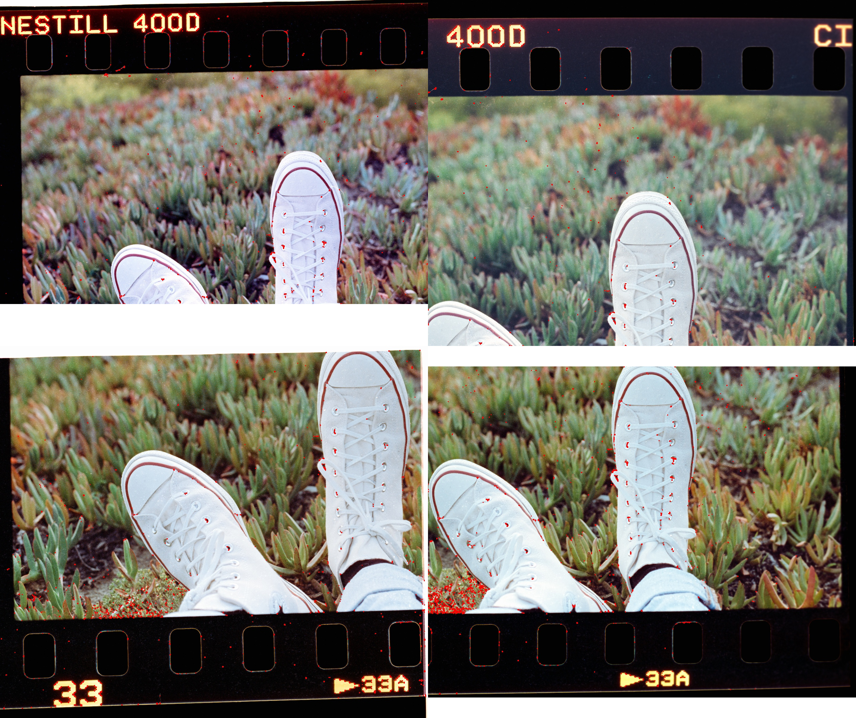Figure 5

Feature Matching

Before we can align our images, we need some sort of metric to determine how well a certain transformation works. We’ll dig more into what these metrics are later, but for now we’d like to be able to say that two features (i.e. corners) on the source and target images correspond to the same feature (with some degree of confidence).

The first step in this process is coming up with some way to identify features - we’ll call this a descriptor. A descriptor can be anything as simple as the literal pixels that make up a corner, or contain more complex information such as the gradients, normalized gradient magnitudes, or aggregate pixels around the corner. In our specific instance, just using a 5x5 window around each feature is sufficient, as we know from the problem that none of our images are rotated (i.e. each image will be a planar transformation of one another).

Next, we need to associate descriptors in our source image with descriptors in our target image. This is actually much simpler than it sounds - we can utilize a brute-force algorithm here which compares descriptors based on an L2 norm. For the top two images in Figure 5 for example, the following matching appears

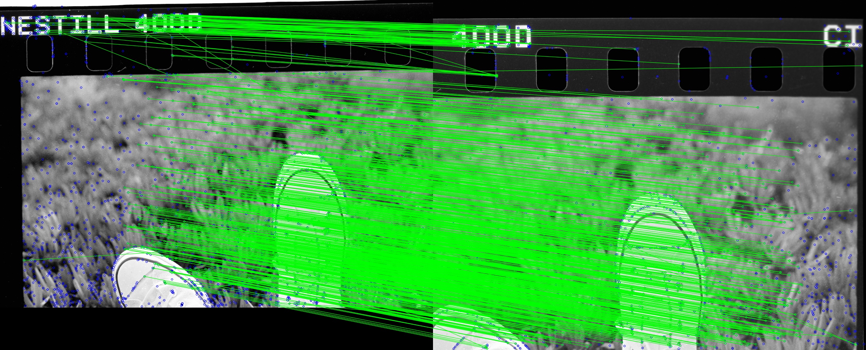Figure 5

Computing the transformation

This is the final step of our algorithm. At this point we’ve done the following operations:

• Computed \(I_x\) and \(I_y\) as approximations of the horizontal and vertical gradients our image using the Sobel kernel
• Computed a matrix \(M\) which represents the covariance of \(I_x\) and \(I_y\) at each pixel
• Reduced \(M\) into a matrix of single values using the Harris corner detector defined by \(R(x,y) = \text{det}(M(x,y)) - k(\text{trace}(M(x,y))^2\).
• Described each corner from the previous step using the neighboring 5x5 pixels
• Matched the descriptors from the previous step using a brute-force algorithm and an L2 norm.

Now all that’s left is to compute the actual transformation that “most properly” overlays the features matched in the previous step.

Linear Least Squares

As is the case with just about any “best-fit” problem, let’s start by formalizing an error function and work our way backwards to understand the solution. Suppose, for now, that we have some function \(f(x_i, p)\) which translates some point \(x_i\) in our source image to a point in the target image based on some parameters \(p\) (we’ll worry about those in a minute). Using the L2 norm, or linear-least squares, this the error is given by the following equation

In other words, we want to find \(\hat{p}\) such that

To solve this equation (in the case of a translation), we can re-write the transformation as the following matrix operation

As such, our goal is to find \(t\) for \(At = b\) which minimizes \(\lvert\lvert At - b\rvert\rvert^2\). Consider the following:

This is pretty cool, since it means that we have a deterministic way to compute the transformation.

Unfortunately, linear least squares performs quite poorly for our use case. To motivate this, let’s see what output LLS produces for the matches given in Figure 5.

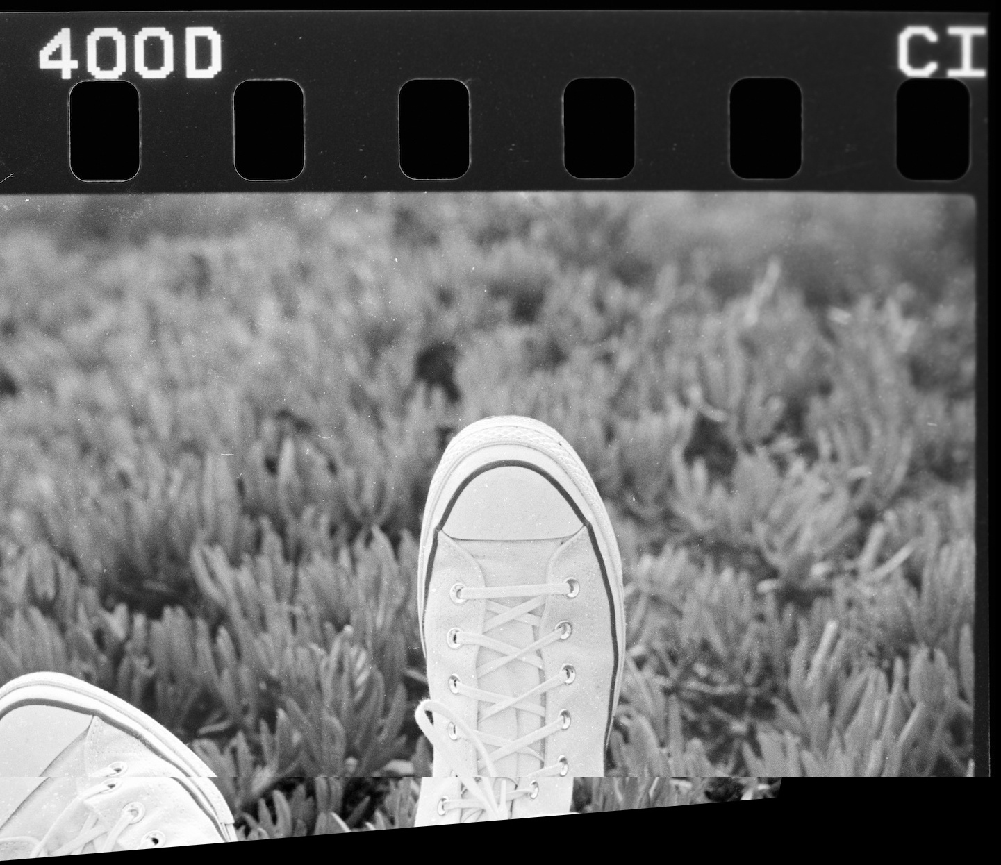Figure 6

The problem here is that LLS does not deal well with outliers. A common theme in computer vision is that our data is never perfect, and as such we should adjust our algorithms to anticipate this. What’s happening in this case, for example, is that certain features which might actually be quite far apart are “matched”, meaning that they’re penalizing our algorithm for our very own mistake.

RANSAC

It’s time for the final piece of the puzzle - RANSAC (RANdom Sample Concensus). RANAC is an algorithm which allows us to compute some sort of transformation with the understanding that there will be outliers. Generally speaking, the algorithm works as follows:

func ransac()
 while model is not found with high confidence
  sample n points randomly from our data
  solve for model parameters using ONLY this data
  score the accuracy using ONLY a set of inliers given by some delta

Visually speaking, you can picture RANSAC as working to fit a line to a number of 2-dimensional datapoints. The green dots represent our randomly sampled points used to fit the model. The blue dots are inliers, whereas the red dots are outliers. The value \(\delta\) represents the threshold given for inliers.

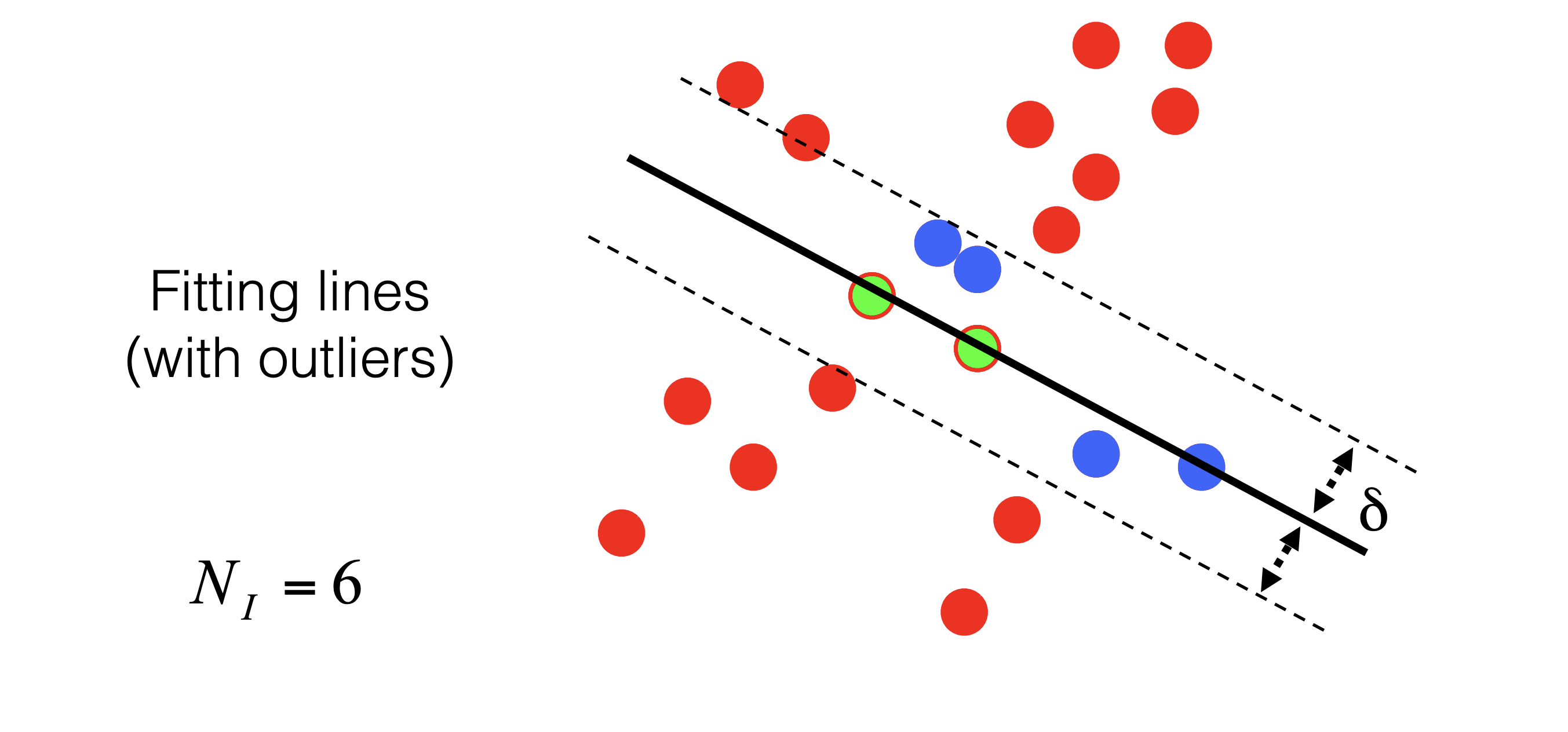Figure 7, courtesy of Kris Kitani at CMU

Tuning the parameters here depends on your use case, but I don’t find the details there too interesting so I’m going to skip over it. Using RANSAC as our homography function instead of LLS yields the following results for the first two images:

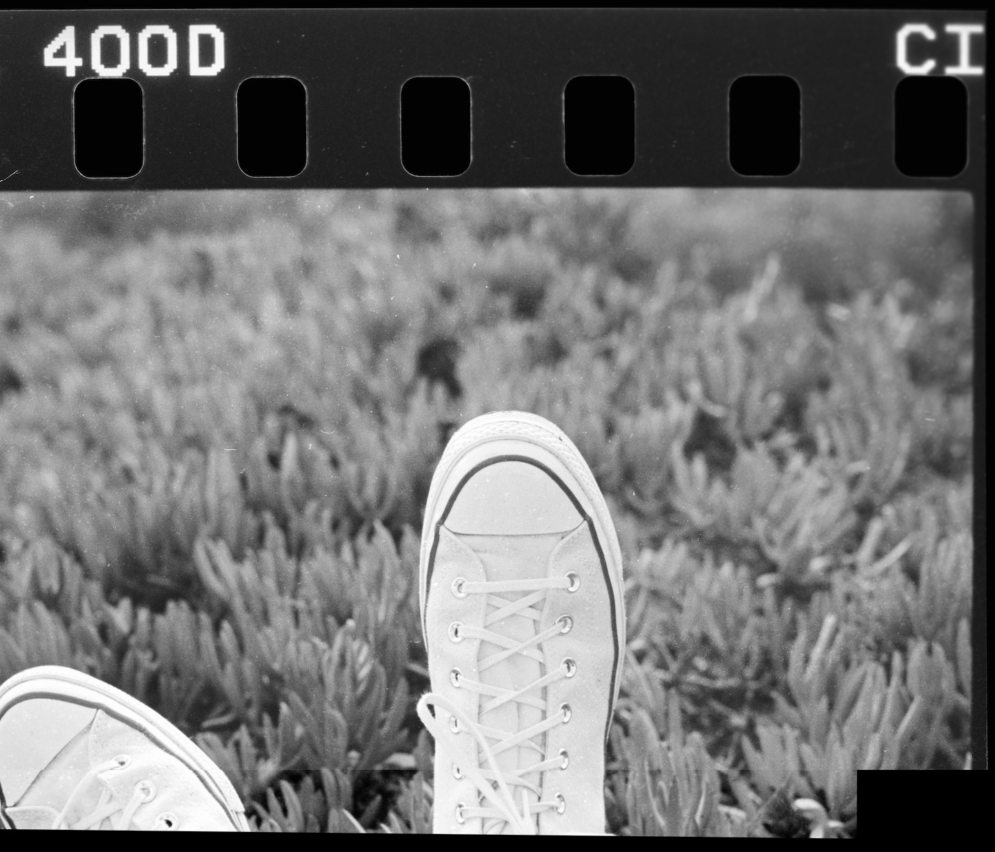Figure 8

Now look at just how nifty that is! Stitching the other images together, doing some minor blending at the boundaries, and bringing back the color yields the following result: